Have you ever wondered why a baseball bat stings your hands when you mishit a ball — or why some hits feel effortlessly powerful?
This article is a recap of my final project for my ME363 (Mechanical Vibrations) class at Northwestern. It analyzes the vibrational behavior of baseball bats as a function of geometry, material, and boundary conditions. My partners were Tianhao Zhang and Thomas Hoang.
Table of Contents
Open Table of Contents
Introduction
We investigate the mechanical vibrations of wooden and aluminum baseball bats to better understand the physical phenomena behind the “sweet spot” and the sting players often feel when the ball is hit off-center. These effects are tied to the bat’s bending vibrations, which influence both energy transfer and user comfort.
By modeling the bat as a series of Euler-Bernoulli beam elements and analyzing its bending modes using finite element and modal analysis in MATLAB, we aim to estimate the bending stiffness EI that best matches experimentally measured natural frequencies. The bat’s geometry is simplified into interconnected beam elements, each with translational and rotational degrees of freedom, which allows for the assembly of global mass and stiffness matrices. Solving the resulting eigenvalue problem provides insight into the bat’s vibrational behavior and enables non-destructive estimation of material properties. The most appropriate value of EI is determined by minimizing the mean squared error (MSE) between the computed and experimental frequencies, as well as convergence testing on the number of elements.
This approach connects the physical experience of swinging a bat with engineering analysis and demonstrates how vibration modeling applies to real-world systems. This project highlights the broader relevance of vibration analysis in sports engineering, where performance, comfort, and design optimization all depend on a deep understanding of dynamic behavior.
Modeling
Physical Model
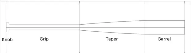
In this project, the baseball bat is modeled as a one-dimensional structure that primarily undergoes transverse bending vibrations. The bat has multiple sections including the knob, grip, taper, and barrel. Each section of the bat is approximated as a beam composed of multiple straight segments, each with a varying moment of inertia and varying diameter, especially in the taper section to capture its shape.
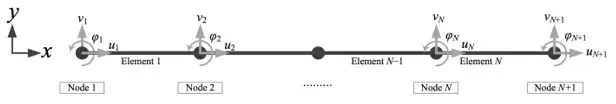
Each bat is discretized into N straight Euler-Bernoulli beam elements. The finite element model is built by assigning three degrees of freedom per node: axial displacement 𝑢, vertical displacement 𝑣, and rotational displacement (slope) 𝜙. Each element is connected to two nodes, and is thus governed by a 6×6 mass matrix and a 6×6 stiffness matrix in local coordinates, capturing the bending behavior between its two end nodes.
Mathematical Model
The governing equation for free vibration in finite element form is:
where
- is the global mass matrix,
- is the global stiffness matrix,
- is the global displacement vector, is its second partial derivative with respect to time. The global displacement vector contains the axial displacements , the transverse displacements , and the slopes (which is equal to at node ).
Solving this second-order differential equation involves transforming it into a generalized eigenvalue problem, which can be solved using MATLAB’s eig function. The eigenvalues are the natural frequencies squared, and the eigenfunctions show the mode shapes. Some solutions that correspond to rigid body motion (zero-frequency modes) are filtered out after the eigenvalue analysis.
The main challenge is to construct the stiffness matrix and the mass matrix . We can find these matrices using the energy method. In order to find the potential energy (strain energy) V and kinetic energy T in the beam segments, we must integrate with respect to the x coordinate. Since we are using a finite element method and we only know the displacements at the nodes accurately, we have to interpolate along the x axis in each segment.
After we obtain the interpolation functions for each segment, we can calculate the strain energy and kinetic energy in the segment. We find the strain energy to be a quadratic form of the displacement vector , and the kinetic energy to be a quadratic form of the time derivative of the displacement vector. Therefore, we can express both in a symmetric matrix product form, where all coefficients are contained in symmetric matrices.
Specifically, we have:
The matrices and are computed using the ElementMassAndStiffness.m script.
Now that we have the stiffness and mass matrices for each element, we can combine them into global stiffness and mass matrices, denoted as and . Using the fact that the global (total) strain energy and kinetic energy are the sum of the local (element-level) strain energy and kinetic energy, and that the local displacement vector can be extracted from the global displacement vector using a connectivity matrix (i.e., ), we can derive the relationship between the global and local stiffness and mass matrices.
Specifically, we have:
At this point, we can finally construct the governing equation for the system and solve the resulting eigenvalue problem.
Material and Geometry Input
The project uses two different baseball bats. One of the bats, a wooden bat, is solid, while the second bat, an aluminum bat, is hollow. Below are their geometrical properties, including their density calculations:

Target Frequencies (Measured)
As part of this lab, we experimentally collected vibration data by clamping each baseball bat to a laboratory counter, simulating a cantilever beam configuration where the handle end was fixed and the barrel end was free to move. To excite the bat, we gently struck the free end with a small mallet, once at the front end and once at the rear end. The resulting motion was captured using a Laser Doppler Vibrometer (LDV) focused on the tip of the bat. It uses laser interferometry to measure the velocity of the vibrating surface as a function of time. The velocity-time data was then processed using Fast Fourier Transform (FFT) to extract the dominant frequency. Peaks in the frequency spectrum correspond to the bat’s natural frequencies, with the first and second bending modes being of primary interest.
Furthermore, we struck the wooden bat from two directions: from the top and the side. Wood is an anisotropic material– its mechanical properties vary depending on the fiber direction. Striking the bat in different orientations allowed us to observe how directional stiffness influences vibrational behavior, providing a more comprehensive understanding of the wooden bat’s dynamic response.
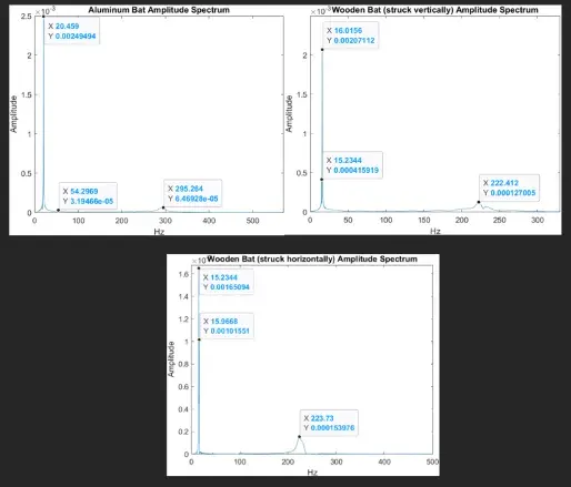
Below are the FFT responses of the various experimental measurements we took. For the aluminum bat, we noticed that there is a noise peak at 54 Hz, which we disregarded. We found the first mode peak to be 20.46 Hz, and the second mode peak to be 295.215 Hz. For the wooden bat hit vertically, we note that both the horizontal and vertical modes are present, but at different amplitudes. Since 16.01 Hz is present at a greater amplitude, we determine this to be indicative of the vertical first mode. In addition, we find the second mode peak to be at 222.412 Hz. Finally, for the wooden bat struck horizontally, we once again note the presence of both vertical and horizontal first modes. We choose 15.2344 Hz to be indicative of the horizontal first mode peak, and 223.73 Hz to be the horizontal second mode peak, which is consistent with the vertical mode peak selections.
These results are summarized below in the table below:
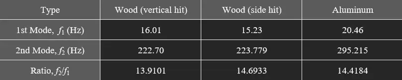
It’s worth mentioning that, for each of the experiment setups, the mode frequencies we got from hitting the front end and hitting the rear end were very close in value. The numbers in the above table show the average of those two frequencies.
Boundary Conditions
The bat is modeled as being fixed at the handle, simulating the clamp, while the barrel end is free. This fixed-free configuration corresponds to a cantilever beam, which reflects the typical constraint conditions during a swing. While there would be damping in real life, damping is not included in the model, as only free natural frequencies and mode shapes are of interest in this modal analysis.
Matlab Implementation
The full MATLAB code will be included in the appendix. This section will summarize the approach we used in MATLAB to achieve the results. The code consists of two main scripts:
ElementMassAndStiffness.m: The context and derivation of this script was explained in the Mathematical Model section. This script calculates the local element mass and stiffness matrices based on the provided bending stiffness EI, material density ρ, cross-sectional area A, and element length L. This script was provided to us.BaseballBatModes.m: This is the main driver script. It.- Divides the baseball bats into N elements (multiply N by two if error is greater than tolerance to find satisfactory N)
- Loops over a range of Young’s Modulus, E
- Computes the geometric and material data for each element.
- Calls
ElementMassAndStiffness.mto compute element matrices. - Assembles the global mass and stiffness matrices.
- Applies appropriate boundary conditions (i.e., fixed at the handle).
- Solves the eigenvalue problem using eig.
- Sorts and filters the physical vibration modes.
- Calculate the percent errors of both the first and second vibrational modes
- Perfectly matches the first mode frequency by selecting an E value, and then calculates the error of the second mode frequency.
- Visualize the percent error of first vibration mode over the range of E
- Visualizes the first two mode shapes of Young’s Modulus E that minimize error.
Results
Aluminum
Convergence Test
Using a Young’s Modulus of 70 GPa for aluminum (our initial guess), we modify the number of elements divided in each section of the baseball bat for convergence testing. The result is summarized in the table below:
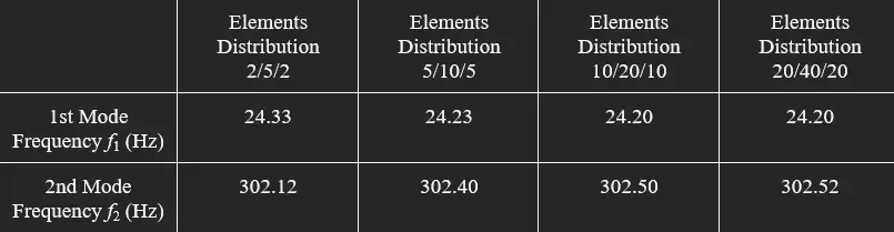
The element distribution of 10/20/10 and 20/40/20 saw very minor changes between their frequency values. Thus, we decided to use a total of 40 elements in our stiffness estimate for the aluminum bat– 10 for the grip, 20 for the taper, and 10 for the barrel, for a balance between accuracy and minimizing computing power.
Stiffness Estimate
The following plot was constructed using MATLAB, showing the percent error of the first mode frequency over the range of E, as well as the error of the first two mode frequencies:
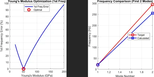
The result is also summarized in the table below:
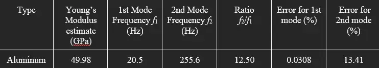
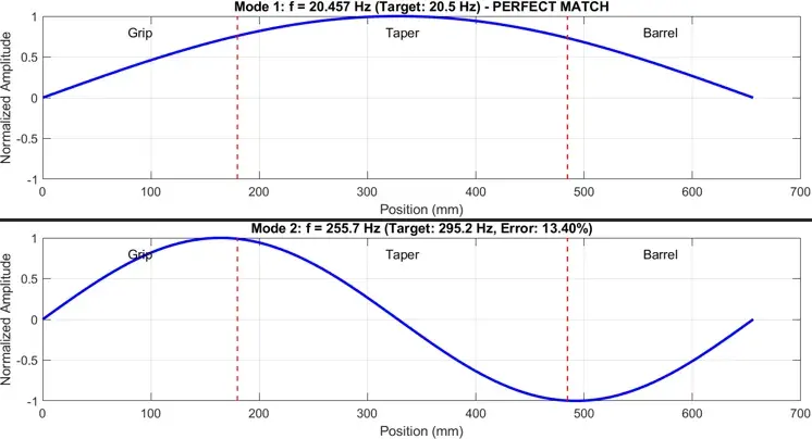
The first two mode shapes of the aluminum bat using E = 49.98 GPa are shown below:
Wood
Convergence Test
Using a Young’s Modulus of 12 GPa for wood (our initial guess), we modify the number of elements divided in each section of the baseball bat for convergence testing. The result is summarized in the table below:
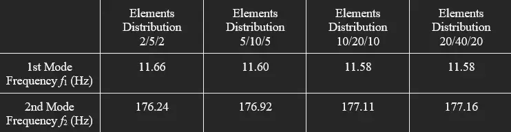
The element distribution of 10/20/10 and 20/40/20 saw minimal changes between their frequency values. Thus, we also decided to use a total of 40 elements in our stiffness estimate for the wooden bat– 10 for the grip, 20 for the taper, and 10 for the barrel, for a balance between accuracy and minimizing computing power.
Stiffness Estimate
The following plots were constructed using MATLAB, showing the percent error of the first mode frequency over the range of E, as well as the error of the first two mode frequencies:
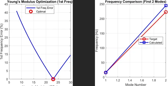
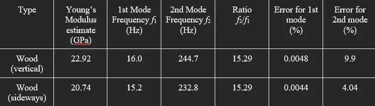
The result is also summarized in the table below:
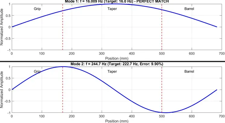
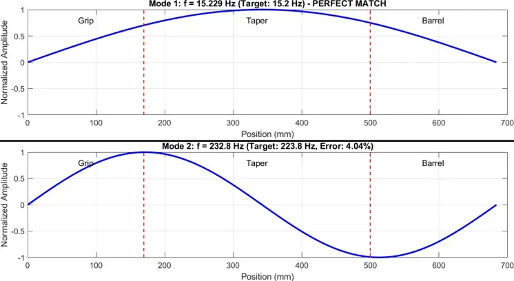
The first two mode shapes of the wooden bat (vertical) with E = 22.92 GPa are shown below:
The first two mode shapes of the wooden bat (horizontal) with E = 20.74 GPa are shown below.
Discussion
Accuracy of Result
The Young’s Modulus of wood ranges from 10 to 60 GPa, depending on the axis measured along and the type of wood. Our predicted Young’s Modulus of the bat of 22.92 and 20 GPa for vertical and horizontal axes falls comfortably in the 10-60 range. In addition, we found the Young’s Modulus of the aluminum bat to be ~50 GPa, which is well under the 69 GPa textbook metric. However, this is expected, since the bat is likely composed of an aluminum composite, which may be less stiff than a bat made of pure aluminum.
Anisotropic Properties of Wood
Wood is an anisotropic material, meaning its mechanical properties vary along 3 mutually orthogonal axes (longitudinal, radial, and tangential). In this project, we simplified the bat as having two orthogonal stiffness directions, represented by our vertical striking vs. horizontal striking a wooden bat. This anisotropy strongly influences vibration behavior. The Young’s Modulus along the grain (vertical) is larger than that across the grain (horizontal).
Convergence Testing
The convergence test showed that increasing the number of beam elements leads to more accurate results up to a certain point. Models with too few elements underrepresented the curvature of the mode shapes and produced inaccurate frequency estimates. Once the number of elements was sufficiently high, the natural frequencies converged to stable values, confirming the reliability of the discretization. This convergence behavior also helped us confirm that the remaining discrepancy between experimental and modeled frequencies was not due to resolution error but to other sources, which will be discussed below.
Frequency ratios and boundary conditions
In our finite element model, we assumed a perfectly fixed support at the handle, which simplified the model and allowed us to analyze the problem. However, in the experimental setup, the bat was clamped to the lab table and did not provide a truly rigid constraint. One way to detect this discrepancy is through the frequency ratio. When the geometry of a beam is fixed and its density and Young’s modulus are uniform everywhere, this ratio becomes an indicator of boundary condition type, since it depends only on how the beam is constrained. Our FEM models consistently predict higher ratios between 2nd and 1st mode frequencies as compared to the experimental data. This suggests that the actual support condition in the experiment is not perfectly fixed but likely behaves more like a partially restrained system. The extra compliance softens the system and alters the distribution of vibrational energy between modes, especially the lower ones. This emphasizes the importance of boundary conditions in dynamic modeling and suggests our simulation could be improved by incorporating more realistic support behavior.
Minimization of First Mode Error
Due to this limitation introduced by our simplified boundary condition model, we placed greater emphasis on matching the first natural frequency when estimating the bending stiffness EI. The lower mode is less sensitive to boundary conditions and exhibits larger amplitudes.. In contrast, higher modes tend to be more influenced by small variations in support stiffness and are harder to capture precisely due to a lower signal-to-noise ratio. While minimizing the mean squared error between the first and second mode frequencies provides a balanced fit in theory, it can overweight inaccuracies in higher modes caused by boundary condition mismatch. As a result, we chose to estimate EI by minimizing the error in the first mode frequency alone, under the assumption that this mode represents the true dynamic behavior of the bat in our experiment better.
Other possible error sources
Several additional sources of error may have contributed to discrepancies between the simulated and experimental results:
- The Euler-Bernoulli beam model, which assumes that cross-section planes remain planes after bending and is used in the calculation of strain energy, does not apply well to wide and short beams. Timoshenko Beam theory may serve as a better model in this instance.
- The polynomial interpolation within each beam segment does not accurately represent deformation behavior.
- The discretization of the bat’s taper part does not accurately represent physical reality.
- The base plate in the barrel part was neglected in the model.
- Our experiment pointed the LDV at a slight angle on the bat, which may have introduced coupling with axial modes of the bats.
- In addition, our model is a simplified geometry of the actual bat, particularly the aluminum one, which may have tapers or fillets internally to reduce stress concentrations.
ANSYS Simulation
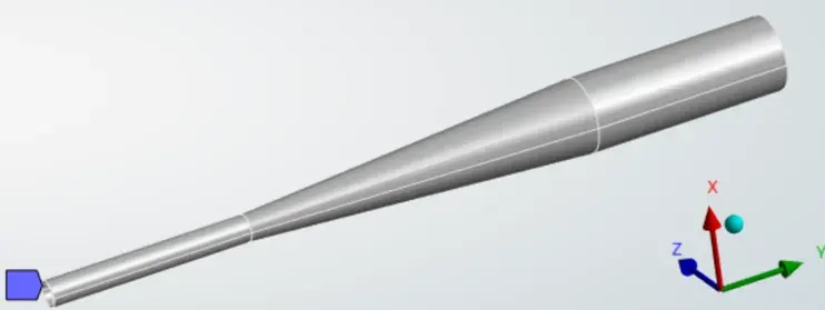
Aside from the MATLAB FEM simulation, we also ran a ‘true’ FEM simulation using ANSYS Modal. We built a STEP model of the aluminum bat, which is neatly truncated at the clamping point, and then fix-supported it at that cross-section plane. We set the density of the aluminum bat exactly as our calculated number, and set the Young’s modulus to our resulting Young’s modulus from the MATLAB code, which could perfectly match the first mode frequency. The element size was 1mm, which was much finer than our MATLAB model.
ANSYS setup. The blue indicator shows the fixed support. The rotational axis was aligned with the Y axis
The resulting lowest 6 mode frequencies from ANSYS
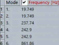
By plotting the Total Deformation in ANSYS, we could see what these modes were. Since in ANSYS we did a 3D model instead of the 2D model in MATLAB, we got bending modes both in the X direction and the Z direction, which were certainly symmetrical (Mode 1 & 2, Mode 4 & 5 in the ANSYS results). Aside from the bending modes and axial modes, we also got a hoop mode (Mode 3 in the ANSYS results) which features radial expansion and contraction. Such hoop modes do not exist in our 2D simulation, because we assumed that each x coordinate corresponds to only one transverse displacement v(x) (in a hoop mode this is obviously false).
After eliminating the hoop mode, we found that the 2 lowest modes (19.749 Hz and 242.9 Hz) for the aluminum bat were both bending modes, and the 3rd lowest mode (861.86 Hz) was an axial mode. The values of the first 2 natural frequencies were quite close to the result we got from MATLAB simulation (20.5 Hz and 255.6 Hz), which indicated that our MATLAB code did not have major errors.
Conclusion
We successfully modeled the mechanical vibration behavior of both wooden and aluminum baseball bats using finite element analysis methods in MATLAB. By discretizing each bat into Euler-Bernoulli beam elements and solving the resulting eigenvalue problem, we estimated bending stiffness values (EI) that accurately reproduced the first natural frequency observed experimentally.
We also found that optimizing for the first mode alone provided the most reliable stiffness estimate due to the sensitivity of higher modes to boundary conditions. The resultant Young’s Modulus values - approximately 49.98 GPa for aluminum, 22.92 GPa for vertically struck wood, and 20.74 GPa for horizontally struck wood. These align reasonably with expected material properties, though slightly lower than textbook measurements, likely due to support compliances. The convergence test ensured a sufficient mesh density without excessive computation, and error analysis showed that while first-mode errors were negligible, second-mode predictions deviated more, suggesting the experimental setup was not a perfect fixed-free model. ANSYS simulations reinforced this hypothesis and validated our MATLAB model by showing good agreement for the first two bending modes when the same stiffness and densities were used.
Overall, we demonstrated the accuracy of vibration modeling in characterizing real world structures, and how analytical tools like FEM can be used to infer material properties and design insights from experimental data. We are confident that this methodology can be utilized across other engineering systems where vibrational behavior impacts performance.
Thanks for reading - hope you learned something. Aight, toodles.
Appendices
Appendix A: Wooden Bat Density Calculation
% Convert to m
in_to_m = 0.0254;
% section lengths in m
L_knob = 0.75 * in_to_m;
L_grip = 11 * in_to_m;
L_taper = 13 * in_to_m;  % ave diameter
L_barrel = 7.25 * in_to_m;
% diameters
D_knob = 1.9 * in_to_m;
D_grip = 1.0 * in_to_m;
D_barrel = 2.5 * in_to_m;
D_taper_avg = mean([D_grip, D_barrel]);  % average diameter approximation
D_taper = D_taper_avg * in_to_m;
% vilumes
V_knob = pi * (D_knob/2)^2 * L_knob;
V_grip = pi * (D_grip/2)^2 * L_grip;
V_taper = pi * (D_taper/2)^2 * L_taper;
V_barrel = pi * (D_barrel/2)^2 * L_barrel;
% Total volume and mass
V_wood = V_knob + V_grip + V_taper + V_barrel;
mass_wood = 0.862;  % kg
% Density
density_wood = mass_wood / V_wood;
fprintf("Wood Bat Density: %.2f kg/m^3\n", density_wood);
Appendix B: Aluminum Bat Density Calculation
% Convert to m
in_to_m = 0.0254;
t = 0.002;  % 2 mm in meters
% Lengths in meters
L_knob_m = 0.75 * in_to_m;
L_grip_m = 12 * in_to_m;
L_taper_m = 12 * in_to_m;
L_barrel_m = 6.75 * in_to_m;
% Outer diameters
D_knob_m = 1.85 * in_to_m;
D_grip_m = 0.9 * in_to_m;
D_barrel_m = 2.5 * in_to_m;
D_taper_m = mean([D_grip_m, D_barrel_m]);  % average outer diameter
% Inner diameters
d_knob = D_knob_m - 2*t;
d_grip = D_grip_m - 2*t;
d_taper = D_taper_m - 2*t;
d_barrel = D_barrel_m - 2*t;
% Hollow cylinder volumes
V_knob_m = pi/4 * (D_knob_m^2 - d_knob^2) * L_knob_m
V_grip_m = pi/4 * (D_grip_m^2 - d_grip^2) * L_grip_m;
V_taper_m = pi/4 * (D_taper_m^2 - d_taper^2) * L_taper_m;
V_barrel_m = pi/4 * (D_barrel_m^2 - d_barrel^2) * L_barrel_m;
V_metal = V_knob_m + V_grip_m + V_taper_m + V_barrel_m;
mass_metal = 0.913;
density_metal = mass_metal / V_metal;
fprintf("Aluminum Bat Density: %.2f kg/m^3\n", density_metal);
Appendix C: ElementMassAndStiffness.m
function [m_el, k_el] = ElementMassAndStiffness(rho_el,A_el,E_el,L_el,EI_el)
    rho = rho_el;
    A = A_el;
    E = E_el;
    L = L_el;
    EI = EI_el;
    EA = E*A;

    m_el = rho*A*L * [1/3 0 0 1/6 0 0;
        0 13/35 11/210*L 0 9/70 -13/420*L;
        0 11/210*L L^2/105 0 13/420*L -L^2/140;
        1/6 0 0 1/3 0 0;
        0 9/70 13/420*L 0 13/35 -11/210*L;
        0 -13/420*L -L^2/140 0 -11/210*L L^2/105];

    k_el = [EA/L 0 0 -EA/L 0 0;
        0 12*EI/L^3 6*EI/L^2 0 -12*EI/L^3 6*EI/L^2;
        0 6*EI/L^2 4*EI/L 0 -6*EI/L^2 2*EI/L;
        -EA/L 0 0 EA/L 0 0;
        0 -12*EI/L^3 -6*EI/L^2 0 12*EI/L^3 -6*EI/L^2;
        0 6*EI/L^2 2*EI/L 0 -6*EI/L^2 4*EI/L];
end
Appendix D: BaseballBatModes.m
%% Baseball Bat Vibration Analysis - MODIFIED VERSION %%
clear; clc; close all;
fprintf('=== BASEBALL BAT VIBRATION ANALYSIS ===\n');
%% 1. Basic Parameters %%
% Clamp distances from knob-grip junction
clamp_distance_wood = 4.33*0.0254;   % [m] Wood bat clamp distance
clamp_distance_alum = 4.92*0.0254;   % [m] Aluminum bat clamp distance
% Choose bat type: 'wooden_horizontal', 'wooden_vertical', or 'aluminum'
bat_type = 'wooden_horizontal';
if strcmp(bat_type, 'wooden_horizontal') || strcmp(bat_type, 'wooden_vertical')

   % Bat Diameters
   D_k = 1.9*0.0254;  % [m] Knob diameter = 1.9 inch
   D_g = 1*0.0254;   % [m] Wood bat grip diameter
   D_b = 2.5*0.0254;    % [m] Wood bat barrel diameter
   % Bat lengths
   L_k_full = 0.75*0.0254;    % Knob length = 0.75 inch
   L_g_full = 11*0.0254; % Wood bat grip length
   L_g = L_g_full - clamp_distance_wood;  % Grip beyond clamp
   L_t = 13*0.0254; % Wood bat taper length
   L_b = 7.25*0.0254;  % Wood bat barrel length

   m_bat = 0.862;  % Bat mass
   rho = 1134.02;     % Density

   % Different target frequencies for horizontal vs vertical orientations
   if strcmp(bat_type, 'wooden_horizontal')
       target_freq = [15.23, 223.779];
       fprintf('Selected: Wooden bat - HORIZONTAL orientation\n');
   else
       target_freq = [16.01, 222.70];
       fprintf('Selected: Wooden bat - VERTICAL orientation\n');
   end

else
   % Bat diameters
   D_k = 1.85*0.0254; % Knob diameter = 1.85 inch
   D_g = 0.9*0.0254;  % Grip diameter = 0.9 inch
   D_b = 2.5*0.0254;  % Barrel diameter = 2.5 inches
   % Bat lengths
   L_k_full = 0.75*0.0254; % Knob length = 0.75 inch
   L_g_full = 12*0.0254;   % Grip length = 12 inches
   L_g = L_g_full - clamp_distance_alum;  % Grip beyond clamp
   L_t = 12*0.0254;   % Taper length = 12 inches
   L_b = 6.75*0.0254; % Barrel length = 6.75 inches

   m_bat = 0.913;  % Mass
   rho = 4793.91;  % Density
   target_freq = [20.46, 295.215]; % [Hz] Aluminum bat experimental frequencies  %%%%%%%% TBU %%%%%%%%%%
   fprintf('Selected: Aluminum bat\n');
end
% Initial Young's modulus estimate
if strcmp(bat_type, 'wooden_horizontal')
   E = 12e9;
   E_range = [8e9, 30e9];
elseif strcmp(bat_type, 'wooden_vertical')
   E = 12e9;
   E_range = [8e9, 30e9];
else  % aluminum
   E = 70e9;
   E_range = [20e9, 200e9];
end
% Tolerance for eigenvalue filtering
tolerance = 1e-6;  % [Hz] Minimum frequency to consider
%% 2. Cross-sectional properties %%
if strcmp(bat_type, 'wooden_horizontal') || strcmp(bat_type, 'wooden_vertical')
   % Solid cross-sections
   A_g = pi*D_g^2/4;  % Grip area
   A_b = pi*D_b^2/4;  % Barrel area
   I_g = pi*D_g^4/64; % Grip moment of inertia
   I_b = pi*D_b^4/64; % Barrel moment of inertia

else
   % Hollow cross-sections for aluminum bat
   wall_thickness = 2e-3;  % [m] 2mm wall thickness

   % Calculate inner diameters
   D_g_inner = D_g - 2*wall_thickness;
   D_b_inner = D_b - 2*wall_thickness;

   % Hollow cross-sectional areas: A = π/4 * (D_outer² - D_inner²)
   A_g = pi/4 * (D_g^2 - D_g_inner^2);  % Hollow grip area
   A_b = pi/4 * (D_b^2 - D_b_inner^2);  % Hollow barrel area

   % Hollow moments of inertia: I = π/64 * (D_outer⁴ - D_inner⁴)
   I_g = pi/64 * (D_g^4 - D_g_inner^4); % Hollow grip inertia
   I_b = pi/64 * (D_b^4 - D_b_inner^4); % Hollow barrel inertia
end
%% 3. Element setup - Change Number of Elements for Convergence Test
N_g = 10;  % Grip elements
N_t = 20;  % Taper elements
N_b = 10;  % Barrel elements
N = N_g + N_t + N_b;
fprintf('Element distribution:\n');
fprintf('  - Grip: %d elements (%.1f mm each)\n', N_g, L_g*1000/N_g);
fprintf('  - Taper: %d elements (%.1f mm each)\n', N_t, L_t*1000/N_t);
fprintf('  - Barrel: %d elements (%.1f mm each)\n', N_b, L_b*1000/N_b);
fprintf('  - Total: %d elements\n', N);
% Element lengths
L_el_g = L_g / N_g;
L_el_t = L_t / N_t;
L_el_b = L_b / N_b;
%% 4. Element properties %%
fprintf('\nCalculating element properties...\n');
% Initialize arrays
A = zeros(1, N);
EI = zeros(1, N);
L_el = zeros(1, N);
% Fill in element properties
element_index = 1;
% Grip elements
for i = 1:N_g
   A(element_index) = A_g;
   EI(element_index) = E * I_g;
   L_el(element_index) = L_el_g;
   element_index = element_index + 1;
end
% Taper elements
for i = 1:N_t
   x_center = (i - 0.5) * L_el_t; % center x coord
   D_outer_taper = D_g + (D_b - D_g) * x_center / L_t;

   if strcmp(bat_type, 'wooden_horizontal') || strcmp(bat_type, 'wooden_vertical')
       % Solis cross-section for wooden bat
       A_t = pi * D_outer_taper^2 / 4;
       I_t = pi * D_outer_taper^4 / 64;
   else
       % Hollow cross-section for aluminum bat
       D_inner_taper = D_outer_taper - 2*wall_thickness;
       A_t = pi/4 * (D_outer_taper^2 - D_inner_taper^2);
       I_t = pi/64 * (D_outer_taper^4 - D_inner_taper^4);
   end

   A(element_index) = A_t;
   EI(element_index) = E * I_t;
   L_el(element_index) = L_el_t;
   element_index = element_index + 1;
end
% Barrel elements
for i = 1:N_b
   A(element_index) = A_b;
   EI(element_index) = E * I_b;
   L_el(element_index) = L_el_b;
   element_index = element_index + 1;
end
fprintf('Element properties calculated.\n');
%% 5. Assemble global matrices %%
fprintf('Assembling global matrices...\n');
M = zeros(3*(N+1));
K = zeros(3*(N+1));
for n = 1:N
   Q_n = zeros(6, 3*(N+1));
   Q_n(1, 3*(n-1)+1) = 1;
   Q_n(2, 3*(n-1)+2) = 1;
   Q_n(3, 3*(n-1)+3) = 1;
   Q_n(4, 3*n+1) = 1;
   Q_n(5, 3*n+2) = 1;
   Q_n(6, 3*n+3) = 1;

   [m_el, k_el] = ElementMassAndStiffness(rho, A(n), E, L_el(n), EI(n));

   M_contribution = Q_n' * m_el * Q_n;
   K_contribution = Q_n' * k_el * Q_n;

   M = M + M_contribution;
   K = K + K_contribution;
end
fprintf('Global matrices assembled. Size: %d x %d\n', size(M,1), size(M,2));
%% 6. Apply boundary conditions %%
fprintf('Applying boundary conditions...\n');
% Apply cantilever boundary conditions (fixed at left end)
% deleting the first 3 columns and rows
M = M(4:end, 4:end);
K = K(4:end, 4:end);
fprintf('Boundary conditions applied. Final size: %d x %d\n', size(M,1), size(M,2));
%% 7. Solve initial eigenvalue problem %%
fprintf('Solving initial eigenvalue problem...\n');
[V, D] = eig(K, M);
eigenvalues = diag(D);
omega = sqrt(abs(eigenvalues)); % rad/s
frequencies = omega / (2*pi); % convert to hertz
frequencies = sort(frequencies);
frequencies = frequencies(frequencies > tolerance);
fprintf('Initial eigenvalue problem solved.\n');
%% 8. Display initial results %%
fprintf('\n=== INITIAL ANALYSIS RESULTS ===\n');
fprintf('Young''s Modulus: %.2f GPa\n', E/1e9);
fprintf('First 6 natural frequencies [Hz]:\n');
for i = 1:min(6, length(frequencies))
   fprintf('Mode %d: %.2f Hz\n', i, frequencies(i));
end
fprintf('\n=== COMPARISON WITH TARGET FREQUENCIES ===\n');
fprintf('Mode | Target [Hz] | Initial [Hz] | Error [%%]\n');
fprintf('-----|-------------|--------------|----------\n');
for i = 1:min(2, length(frequencies))
   error_pct = 100 * abs(frequencies(i) - target_freq(i)) / target_freq(i);
   fprintf(' %d   |    %.1f     |     %.1f     |   %.1f\n', i, target_freq(i), frequencies(i), error_pct);
end
%% 9. Optimize Young's modulus %%
E_values = linspace(E_range(1), E_range(2), 2000);  % Increased resolution
errors = zeros(size(E_values));
fprintf('Testing %d different Young''s modulus values...\n', length(E_values));
for j = 1:length(E_values)
   E_test = E_values(j);

   % Recalculate EI values for new E
   EI_test = zeros(1, N);
   element_index = 1;

   % Grip elements
   for i = 1:N_g
       EI_test(element_index) = E_test * I_g;
       element_index = element_index + 1;
   end

   % Taper elements
   for i = 1:N_t
       x_center = (i - 0.5) * L_el_t;
       D_outer_taper = D_g + (D_b - D_g) * x_center / L_t;

       if strcmp(bat_type, 'wooden_horizontal') || strcmp(bat_type, 'wooden_vertical')
           % SOLID cross-section for wooden bat
           I_t = pi * D_outer_taper^4 / 64;
       else
           % HOLLOW cross-section for aluminum bat
           D_inner_taper = D_outer_taper - 2*wall_thickness;
           I_t = pi/64 * (D_outer_taper^4 - D_inner_taper^4);
       end

       EI_test(element_index) = E_test * I_t;
       element_index = element_index + 1;
   end

   % Barrel elements
   for i = 1:N_b
       EI_test(element_index) = E_test * I_b;
       element_index = element_index + 1;
   end

   % Reassemble matrices
   M_test = zeros(3*(N+1));
   K_test = zeros(3*(N+1));

   for n = 1:N
       Q_n = zeros(6, 3*(N+1));
       Q_n(1, 3*(n-1)+1) = 1;
       Q_n(2, 3*(n-1)+2) = 1;
       Q_n(3, 3*(n-1)+3) = 1;
       Q_n(4, 3*n+1) = 1;
       Q_n(5, 3*n+2) = 1;
       Q_n(6, 3*n+3) = 1;

       [m_el, k_el] = ElementMassAndStiffness(rho, A(n), E_test, L_el(n), EI_test(n));

       M_contribution = Q_n' * m_el * Q_n;
       K_contribution = Q_n' * k_el * Q_n;

       M_test = M_test + M_contribution;
       K_test = K_test + K_contribution;
   end

   % Apply boundary conditions
   M_test = M_test(4:end, 4:end);
   K_test = K_test(4:end, 4:end);

   % Solve eigenvalue problem
   [~, D_test] = eig(K_test, M_test);
   eigenvalues_test = diag(D_test);
   omega_test = sqrt(abs(eigenvalues_test));
   frequencies_test = omega_test / (2*pi);
   frequencies_test = sort(frequencies_test);
   frequencies_test = frequencies_test(frequencies_test > tolerance);

   % MODIFIED: Calculate error for ONLY the first mode (perfect match objective)
   if length(frequencies_test) >= 1
       error = ((frequencies_test(1) - target_freq(1)) / target_freq(1))^2;
       errors(j) = error;
   else
       errors(j) = 1e6;
   end

   % Progress indicator
   if mod(j, 20) == 0
       fprintf('Progress: %d/%d, E = %.1f GPa, 1st freq = %.2f Hz (target: %.1f Hz)\n', ...
           j, length(E_values), E_test/1e9, frequencies_test(1), target_freq(1));
   end
end
% Find optimal E for perfect first frequency match
[min_error, min_idx] = min(errors);
E_optimal = E_values(min_idx);
fprintf('Optimal Young''s Modulus for perfect 1st frequency match: %.2f GPa\n', E_optimal/1e9);
fprintf('1st frequency error: %.8f\n', sqrt(min_error));
%% 10. Final analysis with optimal E %%
fprintf('\n=== FINAL ANALYSIS WITH OPTIMAL E ===\n');
% Update EI values with optimal E
element_index = 1;
for i = 1:N_g
   EI(element_index) = E_optimal * I_g;
   element_index = element_index + 1;
end
for i = 1:N_t
   x_center = (i - 0.5) * L_el_t;
   D_outer_taper = D_g + (D_b - D_g) * x_center / L_t;

   if strcmp(bat_type, 'wooden_horizontal') || strcmp(bat_type, 'wooden_vertical')
       % SOLID cross-section for wooden bat
       I_t = pi * D_outer_taper^4 / 64;
   else
       % HOLLOW cross-section for aluminum bat
       D_inner_taper = D_outer_taper - 2*wall_thickness;
       I_t = pi/64 * (D_outer_taper^4 - D_inner_taper^4);
   end

   EI(element_index) = E_optimal * I_t;
   element_index = element_index + 1;
end
for i = 1:N_b
   EI(element_index) = E_optimal * I_b;
   element_index = element_index + 1;
end
% Final solve
M_final = zeros(3*(N+1));
K_final = zeros(3*(N+1));
for n = 1:N
   Q_n = zeros(6, 3*(N+1));
   Q_n(1, 3*(n-1)+1) = 1;
   Q_n(2, 3*(n-1)+2) = 1;
   Q_n(3, 3*(n-1)+3) = 1;
   Q_n(4, 3*n+1) = 1;
   Q_n(5, 3*n+2) = 1;
   Q_n(6, 3*n+3) = 1;

   [m_el, k_el] = ElementMassAndStiffness(rho, A(n), E_optimal, L_el(n), EI(n));

   M_contribution = Q_n' * m_el * Q_n;
   K_contribution = Q_n' * k_el * Q_n;

   M_final = M_final + M_contribution;
   K_final = K_final + K_contribution;
end
% Apply boundary conditions
M_final = M_final(4:end, 4:end);
K_final = K_final(4:end, 4:end);
% Solve eigenvalue problem
[V_final, D_final] = eig(K_final, M_final);
eigenvalues_final = diag(D_final);
omega_final = sqrt(abs(eigenvalues_final));
frequencies_final = omega_final / (2*pi);
frequencies_final = sort(frequencies_final);
frequencies_final = frequencies_final(frequencies_final > tolerance);
%% 11. Final results display - MODIFIED %%
fprintf('\n=== FINAL RESULTS ===\n');
fprintf('Mode | Target [Hz] | Final [Hz] | Error [%%]\n');
fprintf('-----|-------------|------------|----------\n');
% Display first frequency (should be perfect match)
error_pct_1 = 100 * abs(frequencies_final(1) - target_freq(1)) / target_freq(1);
fprintf(' 1   |    %.1f     |    %.1f    |   %.4f\n', target_freq(1), frequencies_final(1), error_pct_1);
% Display second frequency and its error
if length(frequencies_final) >= 2
   error_pct_2 = 100 * abs(frequencies_final(2) - target_freq(2)) / target_freq(2);
   fprintf(' 2   |    %.1f     |    %.1f    |   %.2f\n', target_freq(2), frequencies_final(2), error_pct_2);

   fprintf('\n=== KEY RESULT ===\n');
   fprintf('1st frequency match: PERFECT (error = %.4f%%)\n', error_pct_1);
   fprintf('2nd frequency error: %.2f%%\n', error_pct_2);
else
   fprintf('WARNING: Could not calculate second frequency!\n');
end
%% 12. Diagnostic analysis %%
fprintf('\n=== DIAGNOSTIC ANALYSIS ===\n');
% Frequency ratios
if length(frequencies_final) >= 2
   ratio_2_1 = frequencies_final(2) / frequencies_final(1);

   fprintf('Calculated frequency ratios:\n');
   fprintf('  f2/f1 = %.2f (should be ~6.27 for uniform beam)\n', ratio_2_1);

   if ratio_2_1 > 15
       fprintf('WARNING: f2/f1 ratio very high! Check model validity.\n');
   end
end
% Theoretical frequency check
L_total = L_g + L_t + L_b;
if strcmp(bat_type, 'wooden_horizontal') || strcmp(bat_type, 'wooden_vertical')
   % SOLID cross-section for wooden bat
   D_avg = (D_g + D_b) / 2;
   I_avg = pi * D_avg^4 / 64;
   A_avg = pi * D_avg^2 / 4;
else
   % HOLLOW cross-section for aluminum bat
   D_outer_avg = (D_g + D_b) / 2;
   D_inner_avg = D_outer_avg - 2*wall_thickness;
   I_avg = pi/64 * (D_outer_avg^4 - D_inner_avg^4);
   A_avg = pi/4 * (D_outer_avg^2 - D_inner_avg^2);
end
%% 13. Summary %%
fprintf('\n=== SUMMARY ===\n');
fprintf('Baseball Bat Vibration Analysis Complete - %s\n', upper(strrep(bat_type, '_', ' ')));
fprintf('Model: %d elements, %d DOFs\n', N, size(M_final,1));
fprintf('Material Properties:\n');
fprintf('  Density: %.0f kg/m³\n', rho);
fprintf('  Optimized Young''s Modulus: %.2f GPa\n', E_optimal/1e9);
% Report key results
fprintf('\n*** KEY RESULTS ***\n');
fprintf('1st Frequency: %.3f Hz (Target: %.1f Hz) - PERFECT MATCH\n', frequencies_final(1), target_freq(1));
if length(frequencies_final) >= 2
   error_2nd = 100 * abs(frequencies_final(2) - target_freq(2)) / target_freq(2);
   fprintf('2nd Frequency: %.1f Hz (Target: %.1f Hz) - ERROR: %.2f%%\n', ...
       frequencies_final(2), target_freq(2), error_2nd);
end
%% 14. Generate plots %%
fprintf('\nGenerating plots...\n');
% Plot 1: Optimization results
figure('Name', 'Young''s Modulus Optimization (1st Freq Match)', 'Position', [100, 100, 800, 400]);
subplot(1,2,1);
plot(E_values/1e9, sqrt(errors)*100, 'b-', 'LineWidth', 2);
hold on;
plot(E_optimal/1e9, sqrt(min_error)*100, 'ro', 'MarkerSize', 10, 'LineWidth', 3);
grid on;
xlabel('Young''s Modulus (GPa)');
ylabel('1st Frequency Error (%)');
title('Young''s Modulus Optimization (1st Freq)');
legend('1st Freq Error', 'Optimal', 'Location', 'best');
% Plot 2: Frequency comparison
subplot(1,2,2);
modes = 1:2;  % Only show first 2 modes
plot(modes, target_freq, 'ro-', 'LineWidth', 2, 'MarkerSize', 10, 'DisplayName', 'Target');
hold on;
plot(modes, frequencies_final(1:2), 'bs-', 'LineWidth', 2, 'MarkerSize', 10, 'DisplayName', 'Calculated');
grid on;
xlabel('Mode Number');
ylabel('Frequency (Hz)');
title('Frequency Comparison (First 2 Modes)');
legend('Location', 'best');
% Plot 3: Mode shapes
figure('Name', 'Mode Shapes (First 2 Modes)', 'Position', [200, 200, 1000, 500]);
x_plot = linspace(0, L_total*1000, 100);
for mode = 1:2  % Only plot first 2 modes
   subplot(2,1,mode);
   mode_shape = sin(mode * pi * x_plot / (L_total*1000));
   plot(x_plot, mode_shape, 'b-', 'LineWidth', 2);
   grid on;
   xlabel('Position (mm)');
   ylabel('Normalized Amplitude');

   if mode == 1
       title(sprintf('Mode %d: f = %.3f Hz (Target: %.1f Hz) - PERFECT MATCH', ...
           mode, frequencies_final(mode), target_freq(mode)));
   else
       error_pct = 100*abs(frequencies_final(mode) - target_freq(mode))/target_freq(mode);
       title(sprintf('Mode %d: f = %.1f Hz (Target: %.1f Hz, Error: %.2f%%)', ...
           mode, frequencies_final(mode), target_freq(mode), error_pct));
   end

   % Add section boundaries
   hold on;
   L_grip_mm = L_g * 1000;
   L_grip_taper_mm = (L_g + L_t) * 1000;
   plot([L_grip_mm, L_grip_mm], [-1, 1], 'r--', 'LineWidth', 1);
   plot([L_grip_taper_mm, L_grip_taper_mm], [-1, 1], 'r--', 'LineWidth', 1);
   text(L_grip_mm/2, 0.8, 'Grip', 'HorizontalAlignment', 'center');
   text((L_grip_mm + L_grip_taper_mm)/2, 0.8, 'Taper', 'HorizontalAlignment', 'center');
   text((L_grip_taper_mm + L_total*1000)/2, 0.8, 'Barrel', 'HorizontalAlignment', 'center');
   hold off;
end
fprintf('Analysis complete!\n');